rescomp: An R package for efficient ODE modelling of resource competition

Andrew D. Letten

rescomp is an R package for generating, simulating and visualising ODE models of consumer-resource interactions. In essence, it is a consumer-resource modelling focused interface to the canonical deSolve package.

Model formulation

All rescomp models take the general form,

\[ \frac{dN_{i}}{dt} = N_{i}(\mu_{i}(R_{1},R_{2},...)-m) \,, \]

\[ \frac{dR_{j}}{dt} = \Psi_{j} (R_{j}) - \sum_{i = 1}^{n}Q_{ij} \mu_{ij}(R_j) N_i \,, \]

where \(N_{i}\) is the population density of consumer \(i\), \(R_{j}\) is the density/concentration of resource \(j\), \(\mu_{i}()\) is the per capita consumer functional response of consumer \(i\), \(m\) is the per capita mortality rate (constant or intermittent), \(\Psi_{j}(R_j)\) is the resource supply function, and \(Q_{ij}\) is the resource quota of consumer \(i\) on resource \(j\) (the amount of resource per unit consumer).

From this general form, different model formulations are distinguished by: i) the number of consumers/resources; ii) the form of the consumer functional response; iii) the mode of resource supply; iv) the type of resource; and v) any non-autonomous behaviour including time dependent model parameters and/or instantaneous changes in consumer/resource density (e.g. in batch transfer).

Consumer equations

The consumer growth function can take one of three forms:

1. linear (type I),

\[ \mu_{ij}(R_{j}) = a_{ij}R_{j} \,, \]

where \(a_{ij}\) is a resource consumption constant.

2. nonlinear type II (aka Monod)

\[ \mu_{ij}(R_{j}) = \mu_{max_{ij}}\frac{R_{j}}{k_{ij} + R_{j}} \,, \]

where \(\mu_{max_{ij}}\) is the maximum growth rate and \(k_{ij}\) is the half saturation constant for consumer \(i\) on resource \(j\).

3. nonlinear type III (sigmoidal),

\[ \mu_{ij}(R_{j}) = \mu _{max_{ij}}\frac{R_{j}^2}{k_{ij}^2 + R_{j}^2} \,. \]

An alternative parameterisation to all three functional responses is to incorporate a consumption efficiency term, \(c_{ij}\). The type I model becomes \(\mu_{ij}(R_{j}) = a_{ij}c_{ij}R_{j}\), and for type II and III, \(a_{ij}c_{ij}\) is substituted for \(\mu _{max_{ij}}\). NB. this functional form is mutually exclusive with the specification of resources quotas in the resource equations, i.e. the \(Q_{ij}\)s are dropped from the resource equations.

Resource equations

The resource supply function, \(\Psi_{j}(R_j)\), can also take several forms. Specifically, either the resources are biological and grow logistically,

\[ \Psi_{j} (R_{j}) = r_{j}R_{j}\left(1-\frac{R_{j}}{K_{j}}\right) \,, \]

where \(r_j\) is the resource intrinsic rate of increase and \(K_j\) is the resource carrying capacity;

Or the resources are supplied to the systems at a fixed concentration and rate (as in a chemostat),

\[ \Psi_{j} (R_{j}) = d(S_{j} - R_{j}) \,, \]

where \(d\) represents the flux of resources into and out of the system;

Or the resources are pulsed intermittently (e.g., in serial transfer - see examples below).

In the case of multiple resources, each resource is either treated as essential to consumer growth following Leibig’s law of the minimum, in which case,

\[ \mu_{i}(R_{1}, R_{2},...,R_{n}) = min(\mu_{i}(R_{1}), \mu_{i}(R_{2}),..., \mu_{i}(R_{n})) \,; \]

or substitutable such that:

\[ \mu_{i}(R_{1}, R_{2},...,R_{n}) = \mu_{i}(R_{1}) + \mu_{i}(R_{2}) + ... + \mu_{i}(R_{n}) \,. \]

Using rescomp

The main user function in rescomp is spec_rescomp(), which facilitates the definition and parameterisation of a consumer-resource model and the specification of simulation parameters. Function arguments include (but are not limited to):

• Number of consumers/resources
• Consumer functional response (type I, II or III)
• Resource dynamic (chemostat, logistic and/or pulsed)
• Resource type (substitutable or essential)
• Continuous or intermittent mortality (e.g., serial transfer)
• Delayed consumer introduction times
• Time dependent growth and consumption parameters

See ?spec_rescomp for all argument options.

Examples demonstrated in this vignette include:

• One consumer (type 2) and one logistically growing resource

• One consumer (type 2) and one continuously supplied resource (i.e. chemostat)

• Two consumers (type 1 and type 2) and one logistically growing resource

• Two consumers (type 1) and two substitutable resources in a chemostat

• Two consumers (type 1) and two essential resources in a chemostat

• Two consumers (type 2) and one externally pulsed resource

  • Continuous mortality
  • Serial transfer in batch culture (intermittent mortality)

• Two consumers (type 2) with time dependent consumption parameters and one continuously supplied resource

• Three consumers (type 1) on three essential resources generating an intransitive loop (i.e. rock paper scissors dynamics).

Additional examples illustrating other options and functionality can be found in the vignette “Reproducing studies in resource competition with rescomp”, including delayed consumer introduction times and specifying a model with consumer resource efficiencies rather than resource quotas.

Type 2 consumer on a logistically growing resource

library(rescomp)

pars <- spec_rescomp(
  spnum = 1, 
  resnum = 1,
  funcresp = "type2",
  mumatrix = matrix(0.12),
  chemo = FALSE,
  resspeed = 3,
  resconc = 2,
  totaltime = 500
)
#> Model properties 
#>  * 1 consumer(s) and 1 resource(s)
#>  * Consumers have type 2 functional responses
#>  * Resources grow logistically
#>  * Mortality is continuous
#> 
#> Simulation properties 
#>  * Simulation time: 500 time steps
#>  * Init state: consumer(s) = [10], resource(s) = [2]

Visualise functional responses with plot_funcresp(). Faceted by resources and time dependent parameterisations (when relevant).

plot_funcresp(pars, maxx = 2)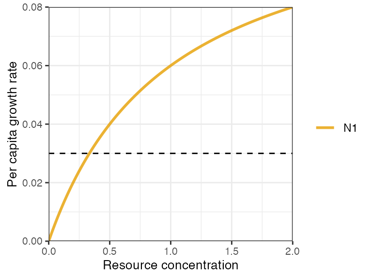

The model can then be simulated with sim_rescomp(). sim_rescomp() is a wrapper to deSolve::ode() that takes the output from spec_rescomp() as its main argument.

m1 <- sim_rescomp(pars)

plot_rescomp() produces a plot of the output dynamics (both consumers and resources).

plot_rescomp(m1)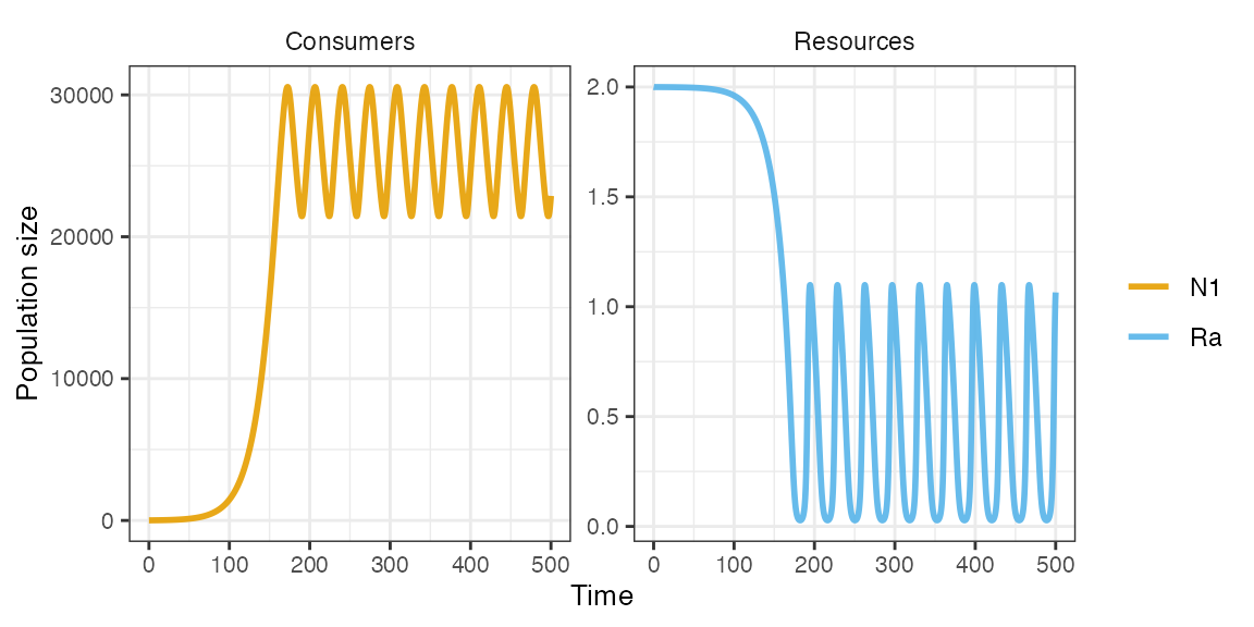

Note the total simulation time and initial state variables specified with spec_rescomp() can be overidden in sim_recomp() with the arguments times and y, respectively. This will nevertheless print a message to the console to check it is intentional. See ?time_vals() for convenient specification of simulation time (and pulsing when used).

m1 <- sim_rescomp(pars, y = c(30000, 1), times = time_vals(200))
#> totaltime in pars will be overidden
#> cinit in pars will be overidden

plot_rescomp(m1)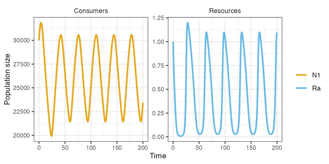

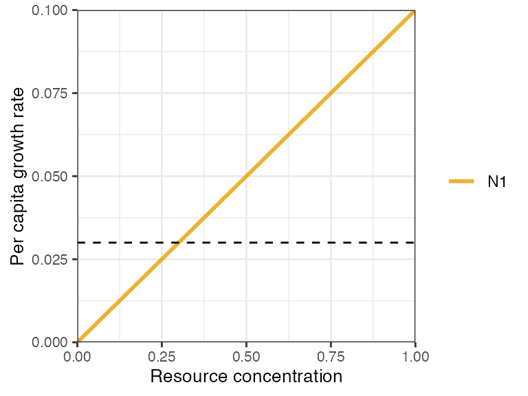
Type 2 consumer on a continuously suppplied resource

pars <- spec_rescomp(
  spnum = 1, 
  resnum = 1,
  funcresp = "type2",
  mumatrix = matrix(0.12),
  resspeed = 0.03,
  resconc = 2,
  totaltime = 300
)
#> Model properties 
#>  * 1 consumer(s) and 1 resource(s)
#>  * Consumers have type 2 functional responses
#>  * Resource supply is continuous (e.g. chemostat)
#>  * Mortality is continuous
#> 
#> Simulation properties 
#>  * Simulation time: 300 time steps
#>  * Init state: consumer(s) = [10], resource(s) = [2]

m1 <- sim_rescomp(pars)

plot_rescomp(m1)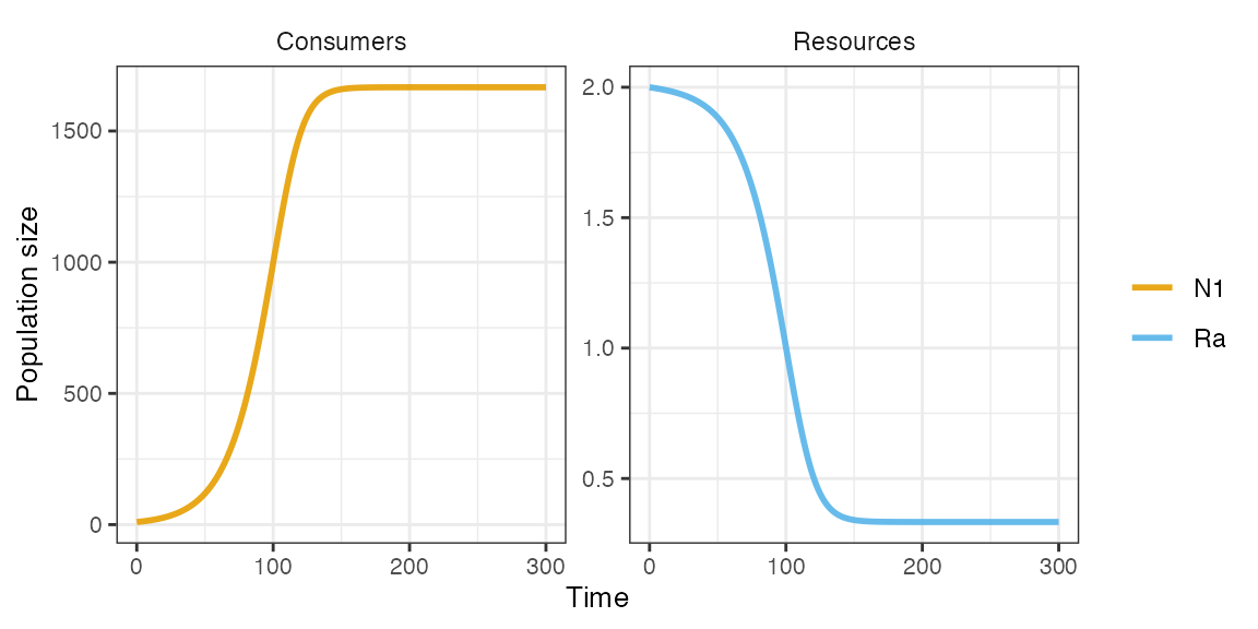

Two consumers (type 1 and type 2) on a logistically growing resource

pars <- spec_rescomp(
  spnum = 2, 
  resnum = 1,
  funcresp = c("type1", "type2"),
  mumatrix = matrix(c(0.35,0.05), 
                    nrow = 2, 
                    ncol = 1,
                    byrow = TRUE),
  kmatrix = matrix(c(1, 0.015), 
                   nrow = 2, 
                   ncol = 1, 
                   byrow = TRUE),  
  chemo = FALSE,
  resspeed = 1,
  resconc = 0.2,
  totaltime = 2000
)
#> Model properties 
#>  * 2 consumer(s) and 1 resource(s)
#>  * Consumers have type 1 or type 2 functional responses
#>  * Resources grow logistically
#>  * Mortality is continuous
#> 
#> Simulation properties 
#>  * Simulation time: 2000 time steps
#>  * Init state: consumer(s) = [10, 10], resource(s) = [0.2]

plot_funcresp(pars, maxx = 0.2)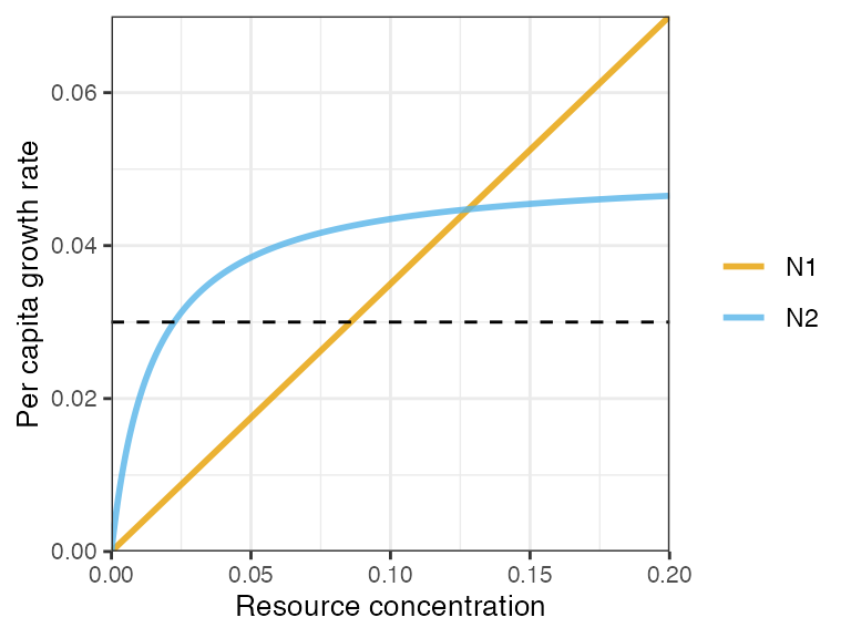

m1 <- sim_rescomp(pars)

plot_rescomp(m1)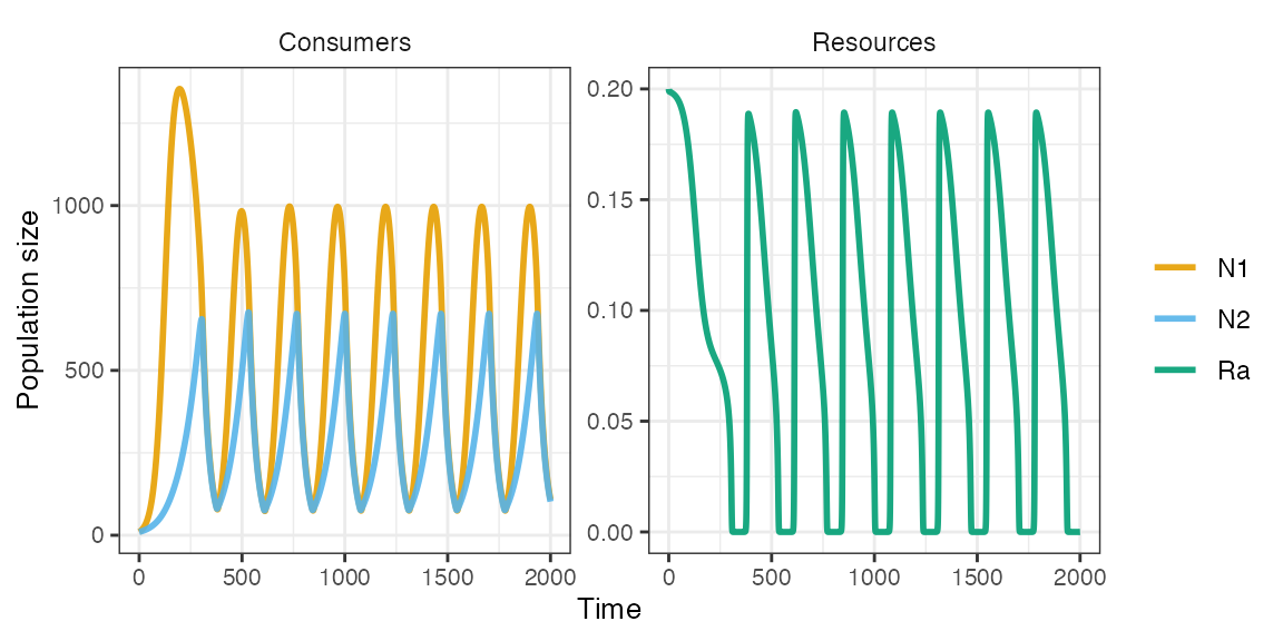

Owing to the trade-off in functional responses (gleaner-opportunist) and resource fluctuations generated by N2, the two consumers are able to coexist.

Two type 1 consumers and two substitutable resources in a chemostat

pars <- spec_rescomp(
  spnum = 2, 
  resnum = 2,
  funcresp = "type1",
  mumatrix = matrix(c(0.09,0.04,
                           0.05,0.08), 
                    nrow = 2, 
                    ncol = 2,
                    byrow = TRUE),
  resspeed = 0.03,
  resconc = 1,
  mort = 0.03,
  essential = FALSE,
  totaltime = 1000
)
#> Model properties 
#>  * 2 consumer(s) and 2 resource(s)
#>  * Consumers have type 1 functional responses
#>  * Resources are substitutable
#>  * Resource supply is continuous (e.g. chemostat)
#>  * Mortality is continuous
#> 
#> Simulation properties 
#>  * Simulation time: 1000 time steps
#>  * Init state: consumer(s) = [10, 10], resource(s) = [1, 1]

plot_funcresp(pars, maxx = 1)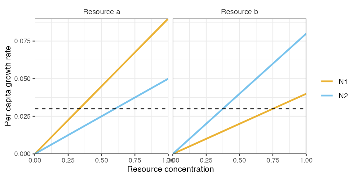

m1 <- sim_rescomp(pars)

plot_rescomp(m1)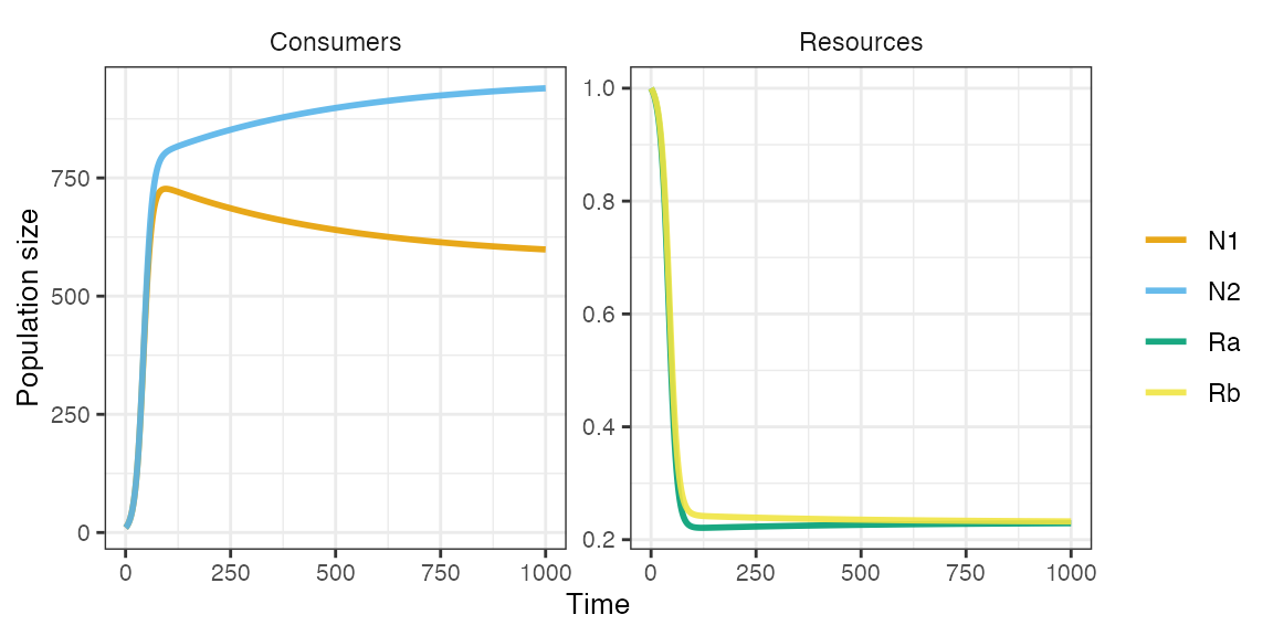

Resource partitioning, where each consumer is a better competitor (lower R*) for a different resource, results in coexistence.

Two type 1 consumers and two essential resources in a chemostat

Using pars$essential = TRUE switches the previous parameteristion to essential resources while keeping all else equal.

pars$essential = TRUE
m1 <- sim_rescomp(pars)

plot_rescomp(m1)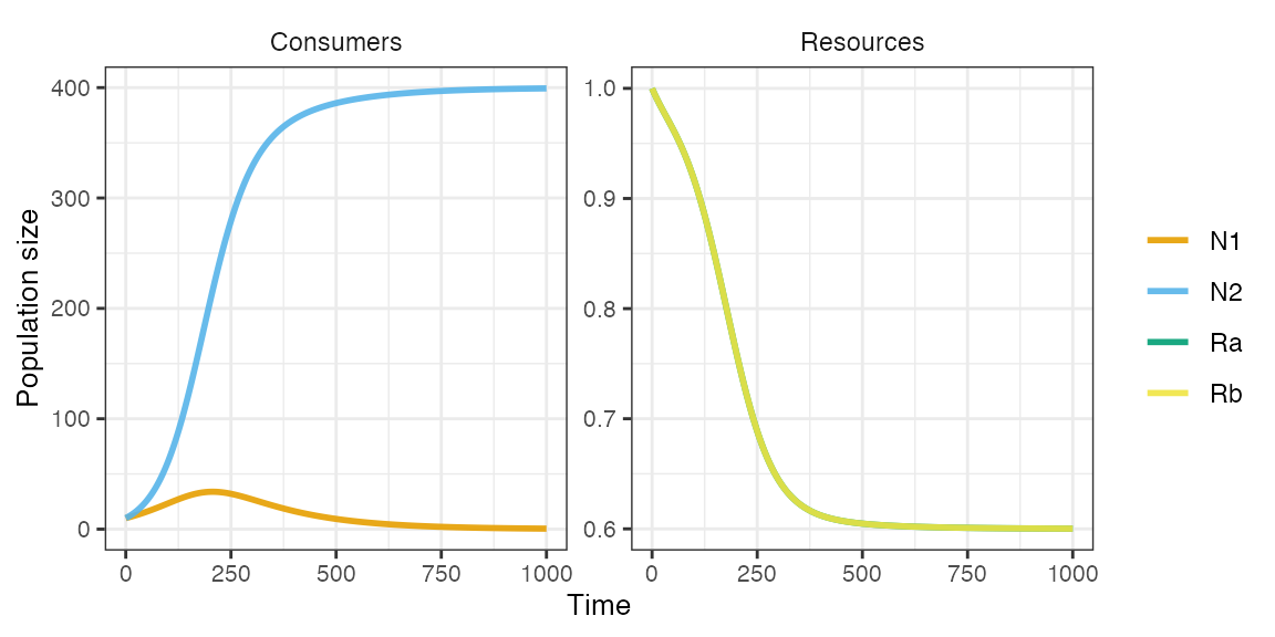 

There is no coexistence now because each species needs to have a larger impact on the resource that is most limiting its growth. For ‘consumer 1’ it is ‘resource b’, whereas for ‘consumer 2’ it is ‘resource a’. We can adjust consumer resource impacts via the resource quota matrix.

pars <- spec_rescomp(
  spnum = 2, 
  resnum = 2,
  funcresp = "type1",
  mumatrix = matrix(c(0.09, 0.04,
                      0.05, 0.08), 
                    nrow = 2, 
                    ncol = 2,
                    byrow = TRUE),
  qmatrix = matrix(c(0.001, 0.005,
                     0.005, 0.001),
                   nrow = 2,
                   ncol = 2,
                   byrow = TRUE),
  resspeed = 0.03,
  resconc = 1,
  mort = 0.03,
  essential = TRUE
)
#> Model properties 
#>  * 2 consumer(s) and 2 resource(s)
#>  * Consumers have type 1 functional responses
#>  * Resources are essential
#>  * Resource supply is continuous (e.g. chemostat)
#>  * Mortality is continuous
#> 
#> Simulation properties 
#>  * Simulation time: 1000 time steps
#>  * Init state: consumer(s) = [10, 10], resource(s) = [1, 1]

m1 <- sim_rescomp(pars)

plot_rescomp(m1)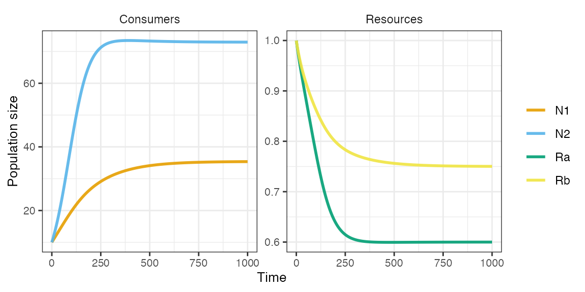 

Two type 2 consumers and one externally pulsed resource (continuous mortality)

External resource pulsing is handled using an auxiliary event function which is generated by the call to spec_rescomp() and passed to sim_rescomp(). The size of the resource pulse is specified as a numeric with the argument respulse in the call to spec_rescomp(). To prevent any other mode of resource supply, resspeed should be set to zero. The frequency of pulsing is set with the pulsefreq argument.

pars <- spec_rescomp(
  spnum = 2, 
  resnum = 1,
  funcresp = "type2",
  mumatrix = matrix(c(0.7,0.05), 
                    nrow = 2, 
                    ncol = 1,
                    byrow = TRUE),
  kmatrix = matrix(c(2, 0.015), 
                   nrow = 2, 
                   ncol = 1, 
                   byrow = TRUE),  
  resspeed = 0, # set to zero for no additional resource supply 
  resconc = 0.2,
  respulse = 0.3,
  pulsefreq = 100 # resource pulse size
)
#> Model properties 
#>  * 2 consumer(s) and 1 resource(s)
#>  * Consumers have type 2 functional responses
#>  * Resource supply is pulsed only
#>  * Mortality is continuous
#> 
#> Simulation properties 
#>  * Simulation time: 1000 time steps
#>  * Resources pulsing every 100 timesteps
#>  * Init state: consumer(s) = [10, 10], resource(s) = [0.2]

plot_funcresp(pars, maxx = max(pars$respulse))

m1 <- sim_rescomp(pars)

plot_rescomp(m1)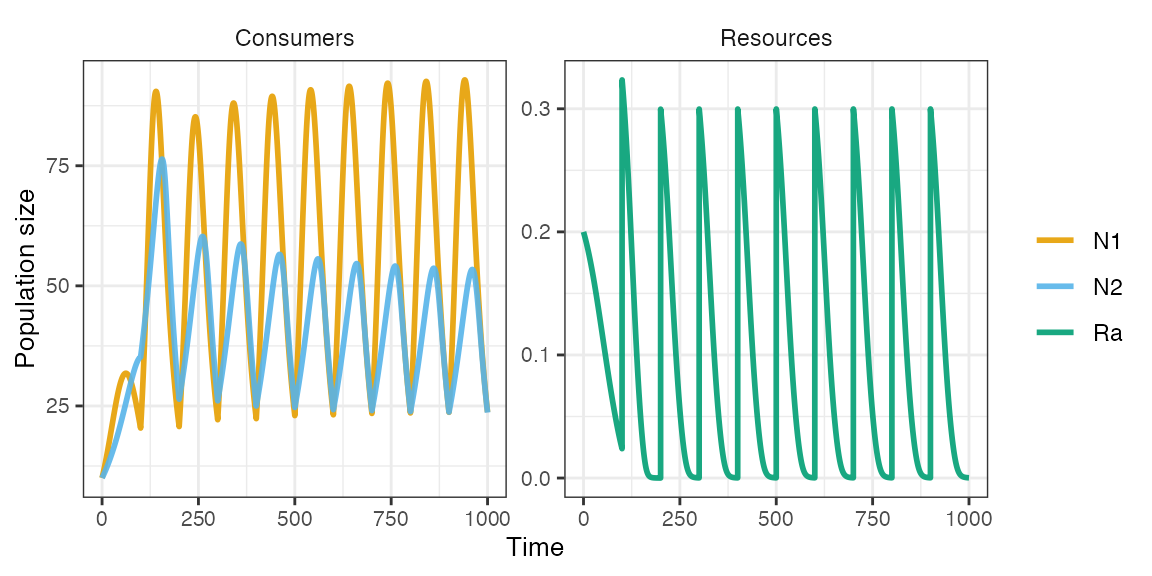

Two type 2 consumers and one externally pulsed resource (serial transfer with pulsed mortality)

Serial transfer in batch culture differs from the above scenario in that resource pulses are typically accompanied by large instantaneous changes in population density. For example, in a serial transfer experiment with bacteria, an experimenter might sample a fraction (e.g. 10%) of the community every 24 hours and inoculate that fraction intro fresh media. As such, the consumer population density immediately following a transfer event will be equal to: \((1-M)N_{i}\), where \(M\) is instantaneous mortality fraction given by mortpulse.

Simulating serial transfer in batch culture is implemented by:

1. Using batchtrans = TRUE in spec_rescomp().
2. Assigning a value from 0 to 1 for the argument mortpulse. This is the fraction of the consumer(s) population instantaneous ‘killed’ at set intervals. Note the transfer fraction = 1 - mortpulse.
3. Setting the serial transfer schedule with the pulsefreq argument (coincident with resource pulse intervals).

Note that the effect of setting batchtrans = TRUE is to enforce fractional sampling of the resource/media in addition to the consumers. As such, immediately after a transfer event the resource concentration will be equal to: \((1-M)R_{j} + MS_{j}\), where \(R\) is the resource concentration prior to transfer, and \(S\) is the resource pulse size given by respulse. To inhibit this behaviour, i.e. to stop fractional sampling of the resource but maintain intermittent mortality use batchtrans = FALSE but still assign a non-zero value for mortpulse.

pars <- spec_rescomp(
  spnum = 2, 
  resnum = 1,
  funcresp = "type2",
  mumatrix = matrix(c(0.2,0.2),
                    nrow = 2, 
                    ncol = 1,
                    byrow = TRUE),
  kmatrix = matrix(c(0.3, 0.2), 
                   nrow = 2, 
                   ncol = 1, 
                   byrow = TRUE),  
  resspeed = 0, 
  resconc = 0.6,
  respulse = 1,
  mort = 0, # set to zero to make the transfer fraction the effective mortality rate
  mortpulse = 0.8,
  batchtrans = TRUE,
  pulsefreq = 100,
)
#> Model properties 
#>  * 2 consumer(s) and 1 resource(s)
#>  * Consumers have type 2 functional responses
#>  * Resource supply is pulsed only
#>  * Mortality intermittent
#> 
#> Simulation properties 
#>  * Simulation time: 1000 time steps
#>  * Resources pulsing and intermittent mortality every 100 timesteps
#>  * Init state: consumer(s) = [10, 10], resource(s) = [0.6]

plot_funcresp(pars, maxx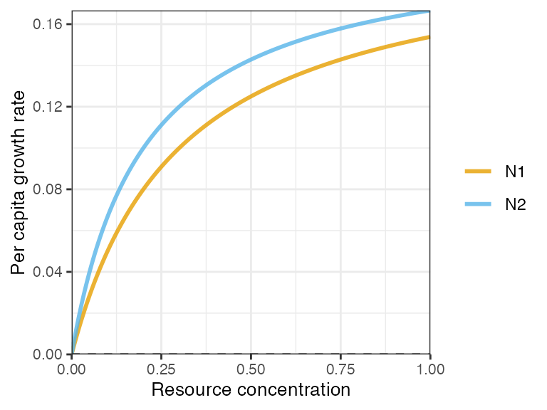 = max(pars$respulse))

m1 <- sim_rescomp(pars)

plot_rescomp(m1)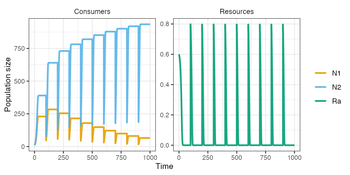

Note, to reproduce the dynamics of a single batch culture experiment (i.e. without serial transfer) as potentially measured via optical density in a plate reader (negligible or unobserved mortality), simply set both resspeed and mort to zero.

pars <- spec_rescomp(resspeed = 0, mort = 0, totaltime = 500)
#> Model properties 
#>  * 1 consumer(s) and 1 resource(s)
#>  * Consumers have type 1 functional responses
#>  * Resources are not supplied?!
#>  * No mortality
#> 
#> Simulation properties 
#>  * Simulation time: 500 time steps
#>  * Init state: consumer(s) = [10], resource(s) = [1]
m1 <- sim_rescomp(pars)

plot_rescomp(m1)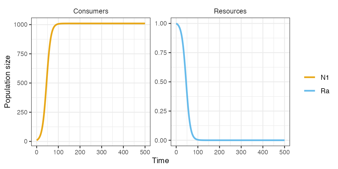

Two type 2 consumers with time dependent consumption parameters and one continuously supplied resource

Using time dependent consumption parameters is appropriate for capturing basic consumer-environment interactions (e.g. differential responses to temperature, pH, antibiotics etc.). Time varying parameters can be implemented in with forcing functions. rescomp provides a convenient means of implementing forcing functions in the background. Two additional arguments are needed in calls to spec_rescomp(): timepars and timeparfreq. timepars should be set to TRUE; timeparfreq adjusts the frequency of switching between ‘environmental states’.

In addition, if time_pars = TRUE, the mumatrix argument in spec_rescomp expects a list containing two matrices, reflecting two different environmental states. At this stage rescomp only handles two states with three interpolation options: i) equal time allotted to each state (default); ii) linear (tpinterp = "lin") interpolation between the two states; iii) sinusoidal (tpinterp = "sine") interpolation between states.

pars <- spec_rescomp(
  spnum = 2, 
  resnum = 1,
  funcresp = "type2",
  mumatrix = list(matrix(c(0.3,0.1), 
                    nrow = 2, 
                    ncol = 1,
                    byrow = TRUE),
                  matrix(c(0.2,0.5), 
                    nrow = 2, 
                    ncol = 1,
                    byrow = TRUE)),
  kmatrix = matrix(c(0.1, 0.1), 
                   nrow = 2, 
                   ncol = 1, 
                   byrow = TRUE),  

  chemo = TRUE,
  resspeed = 0.03,
  resconc = 0.1,
  timepars = TRUE,
  timeparfreq = 50,
  totaltime = 2000
)
#> Model properties 
#>  * 2 consumer(s) and 1 resource(s)
#>  * Consumers have type 2 functional responses
#>  * Resource supply is continuous (e.g. chemostat)
#>  * Mortality is continuous
#>  * Time dependent parameters with instantaneous switching every 50 timesteps
#> 
#> Simulation properties 
#>  * Simulation time: 2000 time steps
#>  * Init state: consumer(s) = [10, 10], resource(s) = [0.1]

plot_funcresp(pars, maxx = max(pars$r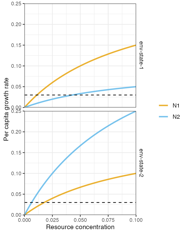esconc))

m1 <- sim_rescomp(pars)

plot_rescomp(m1)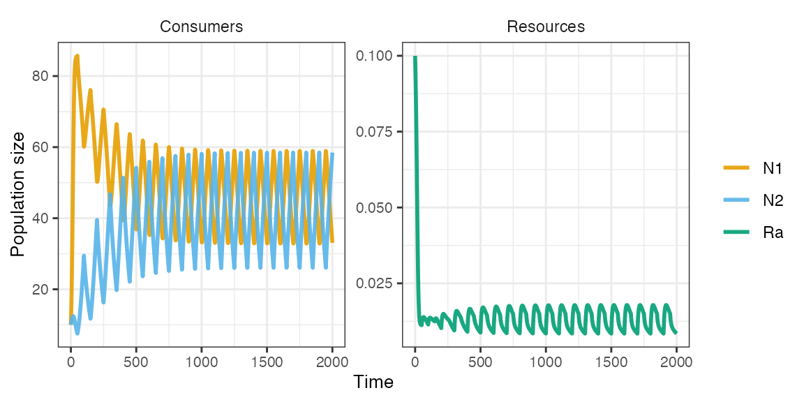

The two consumers coexist due species-specific environmental responses leading to a temporal storage effect.

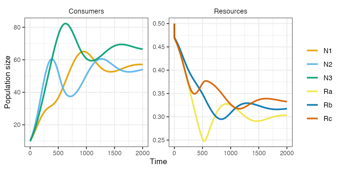
Three type 1 consumers on three essential resources generating an intransitive loop (i.e. rock paper scissors dynamics).

pars <- spec_rescomp(
  spnum = 3, 
  resnum = 3,
  funcresp = "type1",
  mumatrix = matrix(c(0.11, 0.07,  0.045,
                      0.05, 0.11,  0.07,
                      0.07, 0.047, 0.1), 
                    nrow = 3,
                    ncol = 3,
                    byrow = TRUE),
  qmatrix = matrix(c(0.2, 0.7, 0.4,
                     0.4, 0.2, 0.7,
                     0.7, 0.4, 0.2), 
                   nrow = 3,
                   ncol = 3,
                   byrow = TRUE),
  essential = TRUE,  
  chemo = FALSE,
  mort = 0.015, 
  resspeed = 10,
  resconc = 0.5,
  totaltime = 2000
)
#> Model properties 
#>  * 3 consumer(s) and 3 resource(s)
#>  * Consumers have type 1 functional responses
#>  * Resources are essential
#>  * Resources grow logistically
#>  * Mortality is continuous
#> 
#> Simulation properties 
#>  * Simulation time: 2000 time steps
#>  * Init state: consumer(s) = [10, 10, 10], resource(s) = [0.5, 0.5, 0.5]

plot_funcresp(pars, maxx = max(pars$r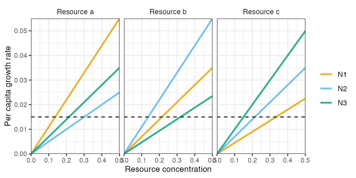esconc))

m1 <- sim_rescomp(pars)

plot_rescomp(m1)