Reproducing studies in resource competition with rescomp • rescomp

This vignette demonstrates the use of rescomp to reproduce several analyses of resource competition from the literature.

library(rescomp)

Huisman and Weissing (1999)

Biodiversity of plankton by species oscillations and chaos. Nature, 402, 407–410

Huisman and Weissing (1999) is notable for showing how oscillations and chaotic dynamics generated by consumers competing for a limited number of resources can foster the coexistence of many more species than there are limiting resources. As a refutation of the competitive exclusion principal, this result provides one solution to the so-called ‘paradox of the plankton’.

The following call to spec_rescomp() specifies a model for 6 species consuming 3 essential resources supplied continuously. The dynamics of the first three species generates a limit cycle. The remaining three species introduced later are able to persist on the resource fluctuations generated by the first three species.

pars <- spec_rescomp(
  spnum = 6,
  resnum = 3,
  funcresp = funcresp_monod(
    mumax = crmatrix(1),
    ks = crmatrix(
      1.00, 0.30, 0.90,
      0.90, 1.00, 0.30,
      0.30, 0.90, 1.00,
      1.04, 0.71, 0.46,
      0.34, 1.02, 0.34,
      0.77, 0.76, 1.07
    )
  ),
  quota = crmatrix(
    0.04, 0.08, 0.14,
    0.07, 0.08, 0.10,
    0.04, 0.10, 0.10,
    0.10, 0.10, 0.16,
    0.03, 0.05, 0.06,
    0.02, 0.17, 0.14
  ),
  ressupply = ressupply_chemostat(
    dilution = 0.25,
    concentration = c(6, 10, 14)
  ),
  mort = 0.25,
  cinit = 0,
  events = list(
    event_set_introseq(
      times = c(0, 0, 0, 1000, 2000, 5000),
      concentrations = c(0.1 + 1/100, 0.1 + 2/100, 0.1 + 3/100, 0.1, 0.1, 0.1)
    )
  ),
  essential = TRUE,
  totaltime = 15000
)

plot_funcresp(pars)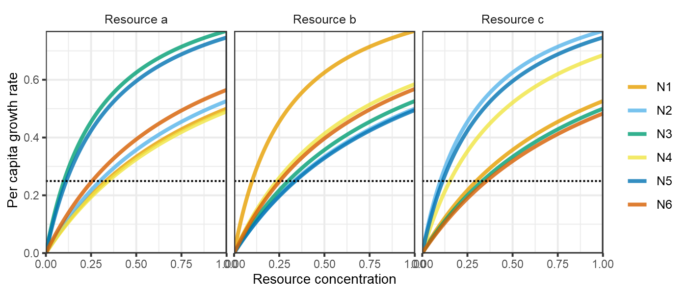

plot of chunk HW1999-funcresps-1c

Be warned the full simulation with 15000 time steps may take a while to run (~2 mins on a laptop with CPU 1.90GHz and 16GB of RAM).

m1 <- sim_rescomp(pars)

plot_rescomp(m1, resources = FALSE)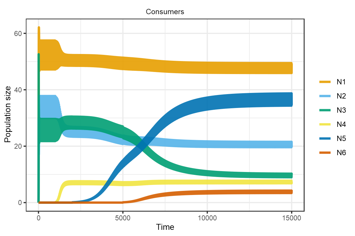

plot of chunk HW1999-dynamics-1c

Reproduces Fig 1c from Huisman and Weissing (1999).

Huisman and Weissing (1999) next showed that chaotic dynamics are common when each consumer has a relatively larger impact on the resource for which it is an intermediate competitor. For example in the model specification below, consumer 1 is an intermediate competitor for resource 4 ( $k_{1,4} = 0.30$ ) but has a larger impact (resource quota) on resource 4 relative to the other four consumers ( $Q_{1,4} = 0.05$ , $Q_{i\neq1,4} = 0.03$ )

pars <- spec_rescomp(
  spnum = 5,
  resnum = 5,
  funcresp = funcresp_monod(
    mumax = crmatrix(1),
    ks = crmatrix(
      0.39, 0.22, 0.27, 0.30, 0.34,
      0.34, 0.39, 0.22, 0.24, 0.30,
      0.30, 0.34, 0.39, 0.22, 0.22,
      0.24, 0.30, 0.34, 0.39, 0.20,
      0.23, 0.27, 0.30, 0.34, 0.39
    )
  ),
  quota = crmatrix(
    0.04, 0.08, 0.10, 0.05, 0.07,
    0.04, 0.08, 0.10, 0.03, 0.09,
    0.07, 0.08, 0.10, 0.03, 0.07,
    0.04, 0.10, 0.10, 0.03, 0.07,
    0.04, 0.08, 0.14, 0.03, 0.07
  ),
  ressupply = ressupply_chemostat(
    dilution = 0.25,
    concentration = c(6, 10, 14, 4, 9)
  ),
  mort = 0.25,
  cinit = c(0.1 + 1/100, 0.1 + 2/100, 0.1 + 3/100, 0.1 + 4/100, 0.1 + 5/100),
  essential = TRUE,
  totaltime = 300
)

plot_funcresp(pars)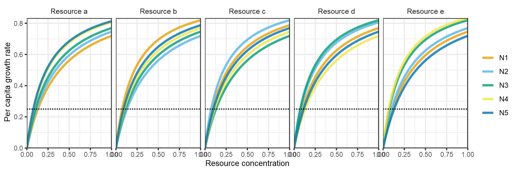

plot of chunk HW1999-funcresp-2

m1 <- sim_rescomp(pars)

plot_rescomp(m1, resources = FALSE, lwd = 1)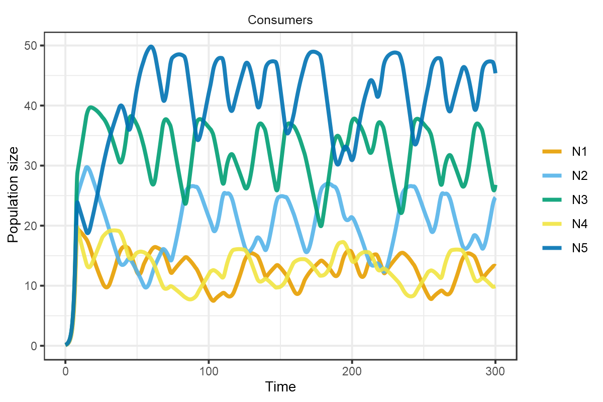

plot of chunk HW1999-dynamics-2a

Corresponds to Fig 2a of Huisman and Weissing (1999).

These chaotic oscillations can in fact foster the coexistence of many more species than limiting resources. In the final example taken from Fig 4 of Huisman and Weissing (1999), 12 species persist on 5 resources.

pars <- spec_rescomp(
  spnum = 12,
  resnum = 5,
  funcresp = funcresp_monod(
    mumax = crmatrix(1),
    ks = crmatrix(
      0.39, 0.22, 0.27, 0.30, 0.34,
      0.34, 0.39, 0.22, 0.24, 0.30,
      0.30, 0.34, 0.39, 0.22, 0.22,
      0.24, 0.30, 0.34, 0.39, 0.20,
      0.23, 0.27, 0.30, 0.34, 0.39,
      0.41, 0.16, 0.07, 0.28, 0.40,
      0.20, 0.15, 0.11, 0.12, 0.50,
      0.45, 0.05, 0.05, 0.13, 0.26,
      0.14, 0.38, 0.38, 0.27, 0.12,
      0.15, 0.29, 0.41, 0.33, 0.29,
      0.38, 0.37, 0.24, 0.04, 0.09,
      0.28, 0.31, 0.25, 0.41, 0.16
    )
  ),
  quota = crmatrix(
    0.04, 0.08, 0.10, 0.05, 0.07,
    0.04, 0.08, 0.10, 0.03, 0.09,
    0.07, 0.08, 0.10, 0.03, 0.07,
    0.04, 0.10, 0.10, 0.03, 0.07,
    0.04, 0.08, 0.14, 0.03, 0.07,
    0.22, 0.14, 0.22, 0.09, 0.05,
    0.10, 0.22, 0.24, 0.07, 0.24,
    0.08, 0.04, 0.12, 0.06, 0.05,
    0.02, 0.18, 0.03, 0.03, 0.08,
    0.17, 0.06, 0.24, 0.03, 0.10,
    0.25, 0.20, 0.17, 0.11, 0.02,
    0.03, 0.04, 0.01, 0.05, 0.04
  ),
  ressupply = ressupply_chemostat(
    dilution = 0.25,
    concentration = c(6, 10, 14, 4, 9)
  ),
  mort = 0.25,
  cinit = 0,
  events = list(
    event_set_introseq(
      times = c(
        0, 0, 0, 0, 0,
        1000, 1000, 1000,
        3000, 3000,
        5000, 5000
      ),
      concentrations = c(
        0.1 + 1/100, 0.1 + 2/100, 0.1 + 3/100, 0.1 + 4/100, 0.1 + 5/100,
        0.1, 0.1, 0.1,
        0.1, 0.1,
        0.1, 0.1
      )
    )
  ),
  essential = TRUE,
  totaltime = 10000
)

plot_funcresp(pars)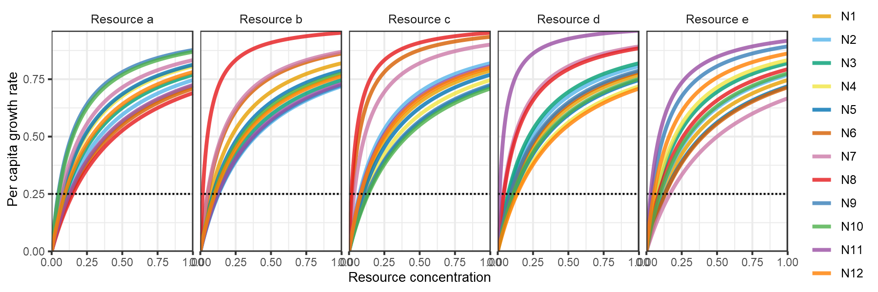

plot of chunk HW1999-funcresp-4

Be warned this simulation will take a relatively long time to run (~8 mins on a laptop with CPU 1.90GHz and 16GB of RAM).

m1 <- sim_rescomp(pars)

plot_rescomp(m1, resources = FALSE, lwd = 0.1)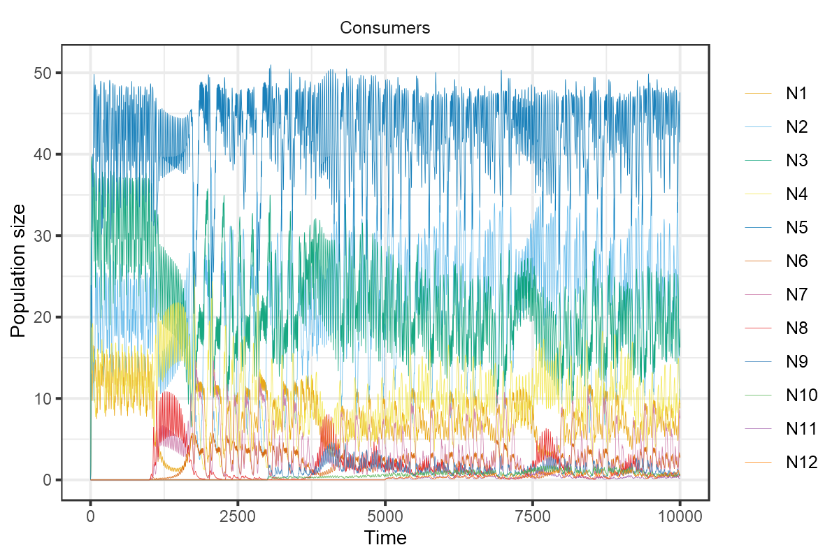

plot of chunk HW1999-dynamics-4

Composite of Figs 4a and 4b from Huisman and Weissing (1999).

Grover (1990)

Resource Competition in a Variable Environment: Phytoplankton Growing According to Monod’s Model. The American Naturalist, 136(6), 771-789.

Grover (1990) coined the term gleaner-opportunist trade-off to describe the trade-off between a consumer with a lower R* (minimum resource requirement) and a consumer with a higher maximal growth rate. Previous studies (including Armstrong and McGehee 1980) had already shown that these two phenotypes could coexist under endogenously generated resource cycling or sinusoidal variation in resource input. In this paper, Grover showed that coexistence via a gleaner-opportunist trade-off extended to periodically delivered resource pulses.

The model comprises a two type two competitors consuming a single resource. When the resource is delivered continuously the gleaner (with a lower R*) predictably excludes the opportunist (with a higher maximum growth rate).

pars <- spec_rescomp(
  spnum = 2,
  resnum = 1,
  funcresp = funcresp_monod(
    mumax = crmatrix(0.5, 0.6),
    ks = crmatrix(0.000001, 0.00001)
  ),
  quota = crmatrix(1/10^8),
  ressupply = ressupply_chemostat(
    dilution = 0.25,
    concentration = 0.0002
  ),
  mort = 0.25,
  rinit = 0.0002,
  cinit = 1000,
  totaltime = 100
)

plot_funcresp(pars, maxx = 0.0001)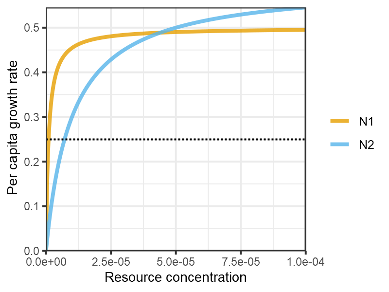

plot of chunk Grover1990-funcresp-4a

Reproduces Fig 1 from Grover (1990). Resource concentration in μmol per ml rather than per L.

mcons <- sim_rescomp(pars)

plot_rescomp(mcons, resources = FALSE, logy = TRUE)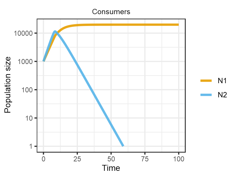

plot of chunk Grover1990-dynamics-4a

Reproduces Fig 4A from Grover (1990).

When the resource is pulsed with high frequency (whilst maintaining the same time averaged resource supply), the gleaner still excludes the opportunist but at a slower rate.

set_pulsing <- function(pars, period) {
  amplitude <- ((0.0002*0.25*period)/(1 - exp(-0.25*period)) - 0.0002)*2
  pars$ressupply <- ressupply_chemostat(
    dilution = 0.25,
    concentration = 0
  )
  pars$rinit <- amplitude
  pars$events <- list(
    event_schedule_periodic(
      event_res_add(amplitude),
      period = period
    )
  )
  return(pars)
}

pars <- set_pulsing(pars, 1)

m1 <- sim_rescomp(pars)
plot_rescomp(m1, resource = FALSE, logy = TRUE)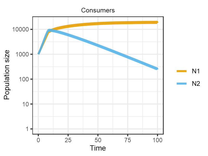

plot of chunk Grover1990-dynamics-4b

Reproduces Fig 4B from Grover (1990).

When the resource is pulsed at an intermediate frequency (again whilst maintaining the same time averaged resource supply), the gleaner and the opportunist coexist.

pars <- set_pulsing(pars, 4)

m4 <- sim_rescomp(pars)
plot_rescomp(m4, resource = FALSE, logy = TRUE)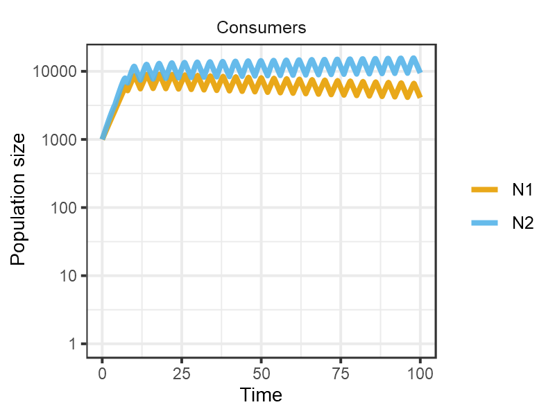

plot of chunk Grover1990-dynamics-4c

Reproduces Fig 4C from Grover (1990).

Finally when the resource is pulsed at low frequency, the opportunist excludes the gleaner.

pars <- set_pulsing(pars, 10)

m10 <- sim_rescomp(pars)
plot_rescomp(m10, resource = FALSE, logy = TRUE)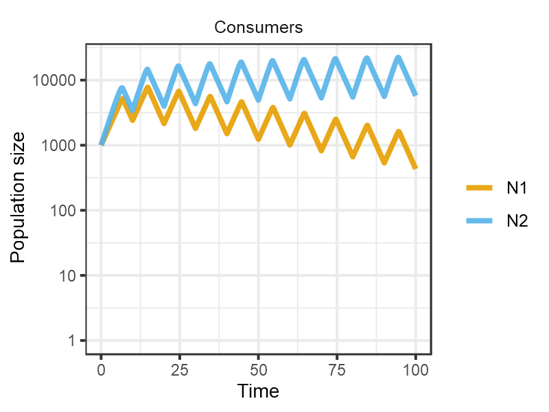

plot of chunk Grover1990-dynamics-4d

Reproduces Fig 4D from Grover (1990).

Armstrong and McGehee (1980)

Competitive Exclusion. The American Naturalist, 115(2), 151-170.

Armstrong and McGehee was one of the first papers to show more than $n$ species can coexist on $n$ resources via endogenously generated cycles in the consumer and resource dynamics. This mechanism for coexistence is indeed commonly referred to as the “Armstrong–McGehee mechanism”.

Unlike the previous examples, Armstrong and McGehee parameterised a two consumer, one resource model using conversion efficiencies in the consumer equations rather than quotas in the resource equations. In spec_rescomp() this is implemented via the specification of an effmatrix rather than a qmatrix. The below code illustrates the model simulation presented by the authors in Figure 1 of their paper.

# TODO: Update this example to the latest version.
# pars <- spec_rescomp(
#   spnum = 2,
#   resnum = 1,
#   funcresp = c("type2", "type1"),
#   mumatrix = matrix(c(0.5, 0.003),
#                     nrow = 2,
#                     ncol = 1,
#                     byrow = TRUE),
#   kmatrix = matrix(c(50, 1),
#                    nrow = 2,
#                    ncol = 1,
#                    byrow = TRUE),
#   effmatrix = matrix(c(0.3, 0.33),
#                    nrow = 2,
#                    ncol = 1,
#                    byrow = TRUE),
#   mort = c(0.1, 0.11),
#   chemo = FALSE,
#   resspeed = 0.1,
#   resconc = 300,
#   totaltime = 600,
#   cinit = c(1,0.01),
#   rinit = 100,
#   introseq = c(0,194)
# )

Because the two consumers were specified with slightly different density independent mortality rates, it is more informative to plot the functional responses using the madj = TRUE argument.

# plot_funcresp(pars, maxx = 200, madj = TRUE)

Corresponds to Fig 2 from Armstrong and McGehee (1980).

With the functional responses adjusted for species specific mortality rates it is clear that intersection of the functional responses lies above both species R*. As shown below, this is harder to interpret when using the default option for plot_funcresp where the two different mortality rates are plotted alongside their functional responses.

# plot_funcresp(pars, maxx = 200)

Simulations show that the species with the nonlinear functional response generates limit cycles upon which the species with the linear functional response is able to persist.

# m1 <- sim_rescomp(pars)

# plot_rescomp(m1)

Corresponds to Fig 1 from Armstrong and McGehee (1980). The paper states that the model was initated with R = 400, but here it is started with R = 100 to provide as close as possible correspondence to the original figure.